
Introduction
The following document will guide you through the required steps to perform a basic analysis in Paintomics. In a nutshell, each process has 3 major steps:
- Upload your data.
- Review initial matching results and configure metabolite assignment, if required.
- Visualization of final results.
However, before starting to use the application you must choose between starting an anonymous session or continuing with an user account, which provides many benefits, read more about them.
Step 1: upload data
The main page shows a data uploading form with 2 sections. In the first one a combobox (Figure 1.A) is provided to allow you to select the organism from an alphabetically ordered list, supporting partial filtering by writing in it. If the species is not present you can use the link to request it and we will install it as soon as possible.
The second section allows you to select analysis databases (Figure 1.B). For some species, more than one database might be available.
The third section contains two parts. In the right one (Figure 1.D) you can enter the input data for each omic to include in the analysis. For doing so the "Browse" button opens a menu with 3 options:
- Upload file from my PC: conventional approach to select the file from your computer.
- Use a file from 'My data': only available for registered users. Read more at Cloud Drive section.
- Clear selection: reset the selected file, if any.
By default "Gene expression" and "Metabolomics" omics are provided, but in the left side (Figure 1.C) you can add more by clicking the  icon; in a similar way, the
  icon allows to undo the action. You can add more than one omic of the same type, provided they have different names. Some options are simple shortcuts with predefined names (like "Proteomics") and will disappear from the list after adding them, unlike the generic ones (like Region based omic).
An important setting is the type of enrichment to perform: based on genes or features. If no selection box is visible, like "Gene expression" or "Metabolomics" shortcuts, is because one default type is assumed by Paintomics. The selection might affect the contingency table used for Fisher test in the pathway enrichment, for instance in proteomics data one protein identifier may match to more than one gene identifier; in feature enrichment type the protein would be counted once, whereas for the gene enrichment type the amount would be the number of genes matched by the protein.
For more information about the configuration options of regulatory and region based omic, read the associated pages in the "Supporting tools" at the left menu of the main Paintomics webpage.
You can read more about the accepted input data in the dedicated page, as well as download the example data here.
Once everything is ready, press the button "Run paintomics" in the upper left corner.
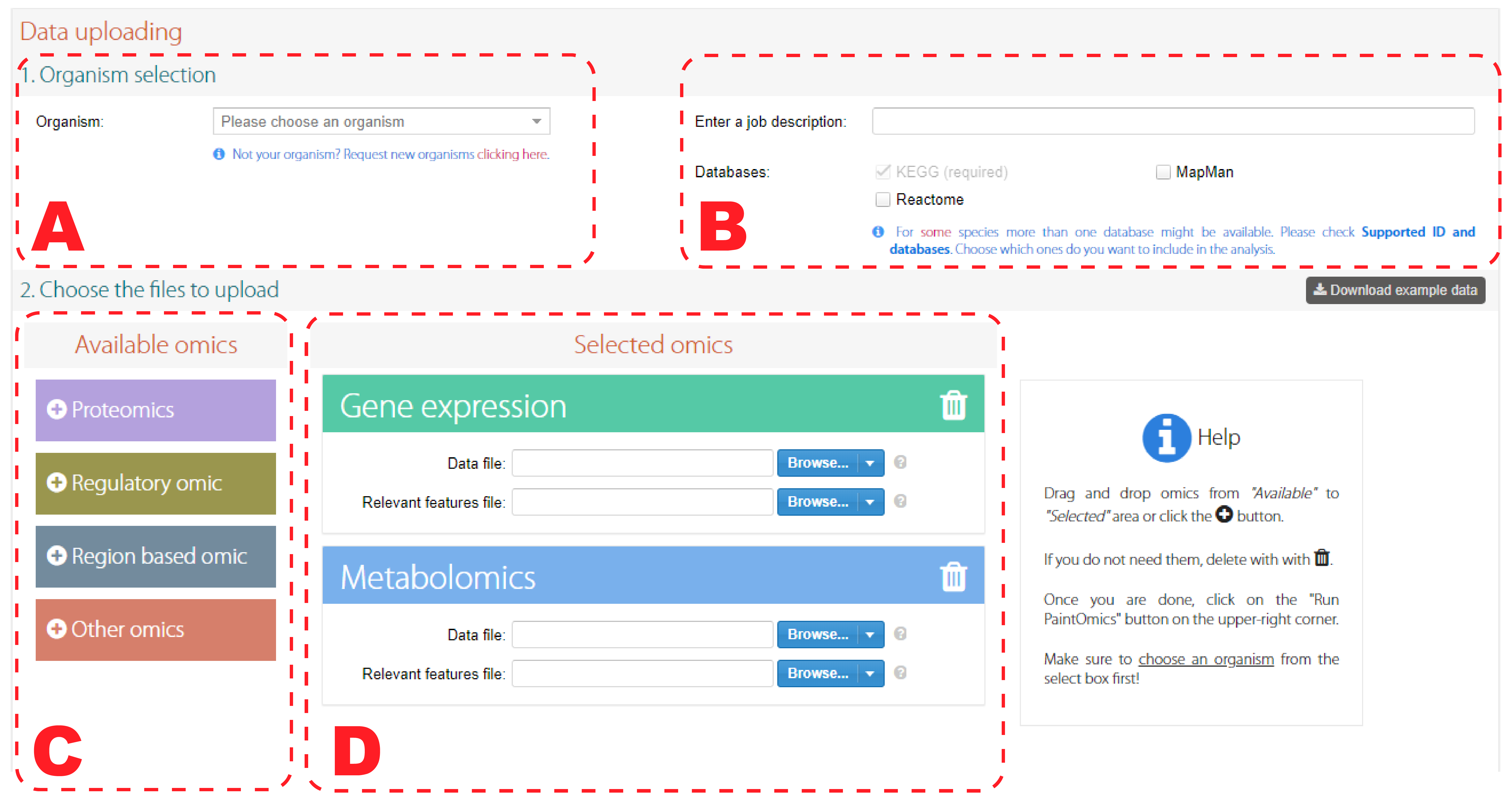
Figure 1. Input data form. Organism selection (A). Database selection (B). Available omics panel (C). Input data for chosen omics (D).
Step 2: matching summaries and metabolite assignment
Paintomics processes your files and offers you different plots showing the results of matching the identifiers of your files to the KEGG/Reactome/MapMan ids (read more here). You can also view diverse information of your data by hovering the data distribution plot with the mouse cursor (Figure 2).
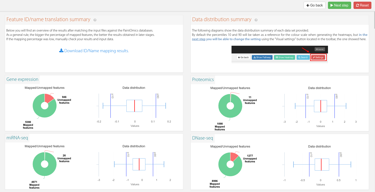
Figure 2. Mapping results and data distribution plots for each omic.
If a compound based omic like metabolomics was provided, an additional section will be available below the previous plots (Figure 3) to review the assignment and correct it if you consider it. Each compound found in your data will show many checkboxes with the candidates.
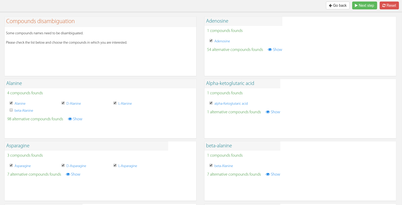
Figure 3. Compound disambiguation.
When you are satisfied with the settings, click "Next step" button.
Step 3: visualizing the results
In the final step Paintomics displays the obtained results offering many configuration options for tweaking the visualization of them.
Pathways summary
This panel shows you the job ID as well as the link you must use to access it. You can also view the number of found pathways and the ones that are significant (p-value lower than 0.05). These counters will be automatically updated based on your filtering options and p-value selection, using by default the Fisher combined method in cases with more than one omic.
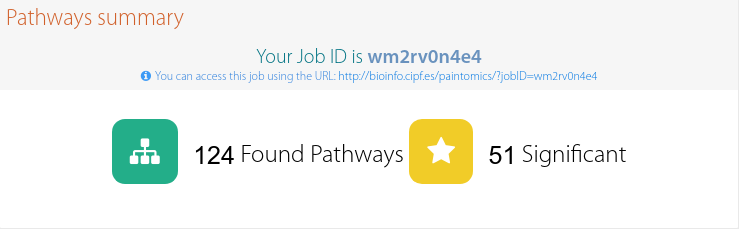
Figure 4. Summary panel showing the job ID as well as the found pathways.
Databases summary
This panel shows you the summary of the pathway enrichment result from multiple databases, and the panel only occurs when multiple databases are used.
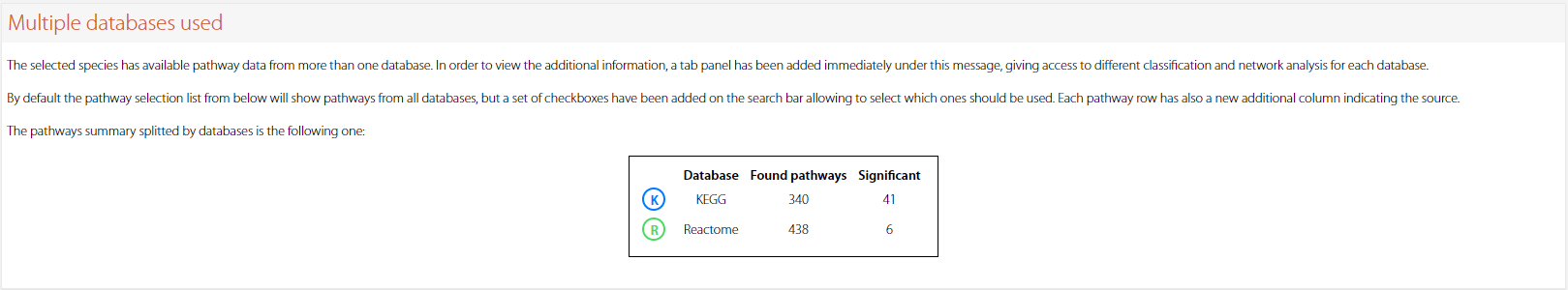
Figure 5. Summary panel showing the job ID as well as the found pathways.
Pathways classification
Each KEGG pathway is associated to a primary category and subcategory (see more here). In this panel you can access that information by expanding the elements of the tree, with options to show or hide individual nodes or entire branches by clicking on the checkboxes or the links that appear when hovering over the options, then the "Apply" button.
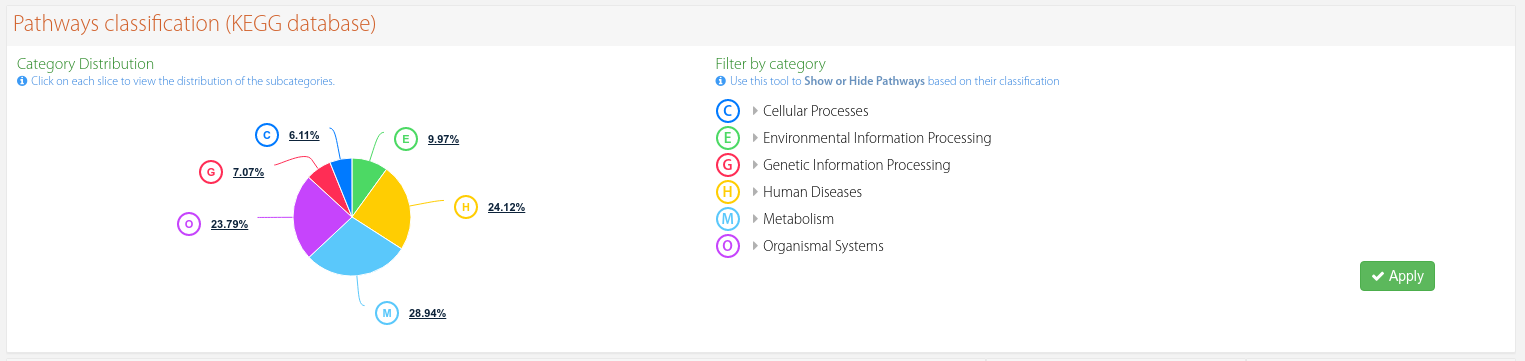
Figure 6. Classification of each KEGG pathway with filtering options.
Pathways network
The pathway interaction network is built according to the process described in this page, in which a more detailed explanation is given.
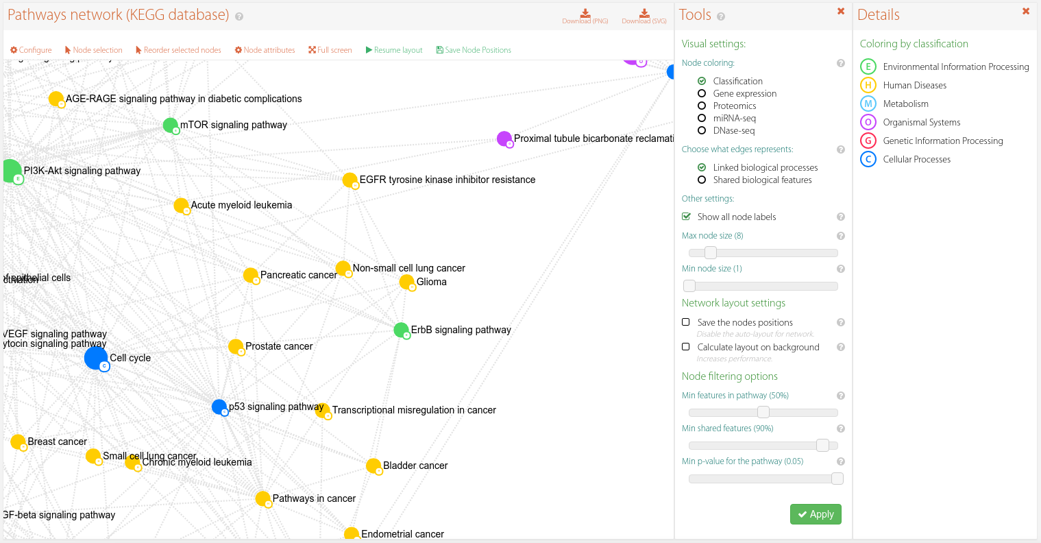
Figure 7. Pathway interaction network.
Pathway enrichment
In the pathway enrichment table you can see every pathway that had at least one match with your data, as explained in this page.
The header of the table has some filtering options to quickly search through the table. Note that this "live search" is not permanent, will not be saved and will not affect the number of found & significant pathways, unlike filtering by category as explained in the classification panel section.
The visible columns can be individually adjusted by hovering the column block (i.e. "Significance tests"), then clicking at the arrow that will appear on the right side. Depending on the job there can also be some additional select boxes to change the method for adjusted p-values or the method for combined p-values; in the last case, selecting 'Stouffer' has method will enable the configure button allowing to use of custom weights for the calculation.
Clicking on the paint column icon ( ) will load the detailed pathway view.
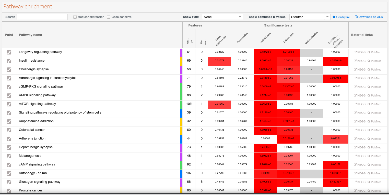
Figure 8. Pathway enrichment table.
Detailed pathway view
The main component of the detailed pathway view is the KEGG diagram showing all the nodes and relationships between them.
Matches are represented by boxes painted over those nodes, containing a heatmap with the record values. One box can have more than one gene or feature associated with it, symbolized by a plus icon. If at least one of these features is significant, a star symbol will also be visible.
Placing the cursor over these boxes will open up a tooltip window expanding the info. If multiple features are associated with it, a "Prev/Next" link will appear in the lower part of that window allowing it to iterate over them.
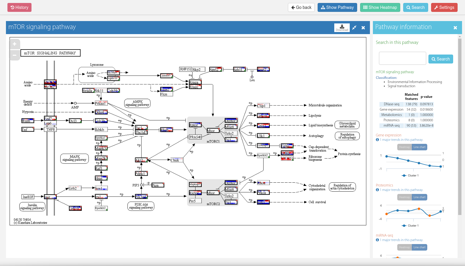
Figure 9. Detailed pathway view.
For any question on PaintOmics, users can send a mail to paintomics4@outlook.com.